Copulas in Climate Risk: Why Extremes Don't Happen Alone

A storm hits the coast. Wind speeds are high but not record-breaking. Rainfall is heavy but not unprecedented. Neither hazard alone would trigger a catastrophic loss. But they arrive together, and the combination produces flooding that neither marginal distribution predicted.

This is compound risk. Events that are individually manageable become catastrophic in combination. It is arguably the central problem in catastrophe modelling, climate adaptation, and reinsurance pricing. And the standard statistical toolkit, fitting marginal distributions to individual hazards, handles it badly.

This post is a visual introduction to copulas, the mathematical framework for modelling dependence between variables. No measure theory, no proofs. If you work in climate risk, catastrophe modelling, or reinsurance, this is the tool you use to answer “how likely are these hazards to happen together?” If you’re coming from climate science, engineering, or just want to understand compound risk better, this should give you the intuition and vocabulary to read the technical literature without getting lost.

The problem with marginals

Climate hazards are routinely assessed in isolation. Wind return periods are estimated from wind data. Flood return periods from rainfall data. Each analysis produces a marginal distribution: a complete description of the behaviour of one variable independently.

The problem is that “independently” is doing a lot of work. If two hazards are positively dependent (high wind tends to coincide with heavy rain during extratropical cyclones), their joint exceedance probability is much higher than the product of their individual probabilities.

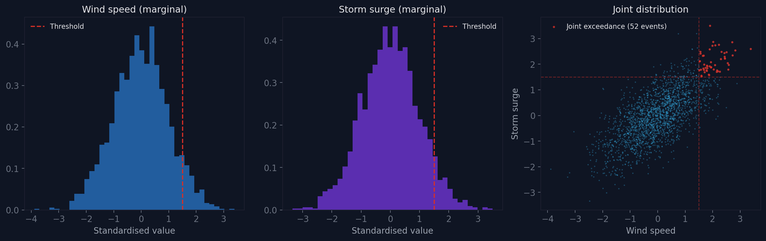
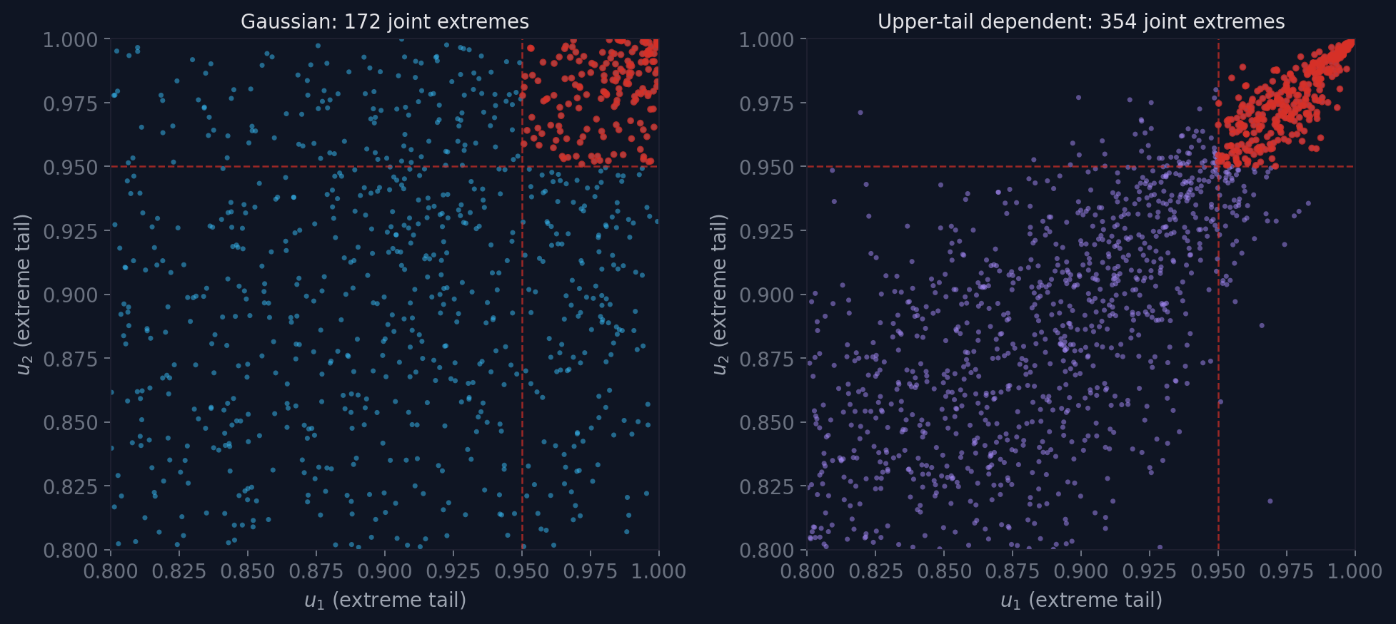
The left two panels look manageable. The right panel tells a different story. Those red dots in the upper-right corner are compound events where both hazards simultaneously exceed their individual thresholds. The marginal distributions, examined alone, don’t see them coming.

If you assume independence, the probability of both hazards exceeding their 95th percentiles simultaneously is 0.05 × 0.05 = 0.0025 (1 in 400). With positive dependence, it can be 1 in 50.

A factor of 8 in risk vanishes from any analysis that treats hazards as independent.

A quick note on distributions

Before we get to copulas, two terms that come up constantly.

A probability distribution describes how likely different values of a variable are. Wind speed, for example, has a distribution: low speeds are common, moderate speeds are frequent, extreme gusts are rare. The shape of the distribution tells you the relative likelihood of each value.

A cumulative distribution function (CDF) is one way to express this. Instead of asking “how likely is a wind speed of exactly 25 m/s?” the CDF asks “what fraction of all observations are at or below 25 m/s?” It outputs a value between 0 and 1. If the CDF at 25 m/s is 0.95, that means 95% of observations fall below 25 m/s. It is a 1-in-20 event. The CDF maps from the variable’s natural units (m/s, mm, °C) to a probability scale.

This mapping is what lets copulas work. By converting every variable to its CDF value, we put everything onto the same [0,1] scale regardless of whether we started with wind in m/s, rainfall in mm, or temperature in °C. That is the probability integral transform, and it is the key step in the copula machinery.

Sklar’s theorem and the copula decomposition

The mathematical foundation for separating dependence from marginal behaviour is Sklar’s theorem (1959). It states:

Every multivariate cumulative distribution function H(x₁, x₂, …, xₙ) can be written as:

H(x₁, …, xₙ) = C(F₁(x₁), …, Fₙ(xₙ))

where F₁, …, Fₙ are the marginal CDFs and C is a copula function.

Conversely, any set of marginals combined with any copula produces a valid joint distribution. The copula C: [0,1]ⁿ → [0,1] captures the entire dependence structure, completely separated from the marginals.

This decomposition is what makes copulas practical:

1. Fit the marginals independently. GEV for wind, lognormal for surge, gamma for precipitation. This is domain-specific and well-understood.
2. Fit the copula to the dependence structure, using rank-transformed data, pseudo-observations, or parametric maximum likelihood. This is portable across applications.
3. Combine. Any marginals with any copula gives a valid joint distribution. You can swap marginals without refitting the copula, or test different copula families without changing the marginals.

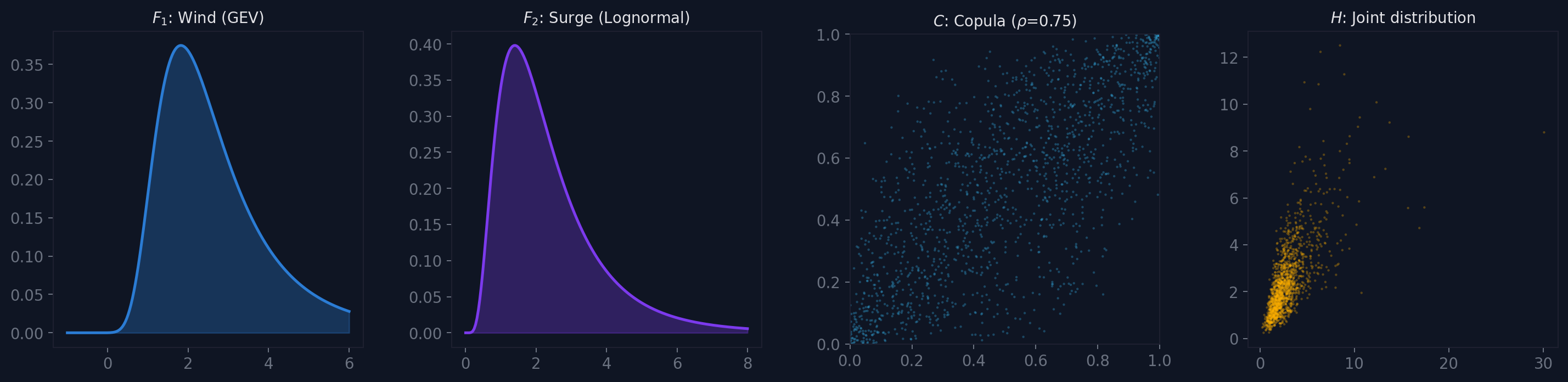
The diagram shows this visually. The GEV wind distribution (left) and lognormal surge distribution (second) are combined through a Gaussian copula (third) to produce the joint distribution (right). The copula determines the shape of the joint scatter, including the clustering and the tail behaviour, while the marginals determine the scale and shape of each individual variable.

What a copula does

A copula operates in uniform space. The probability integral transform converts any continuous random variable X with CDF F into a uniform variable U = F(X) on [0,1]. Applying this to each variable independently removes the marginal structure and leaves only the dependence.

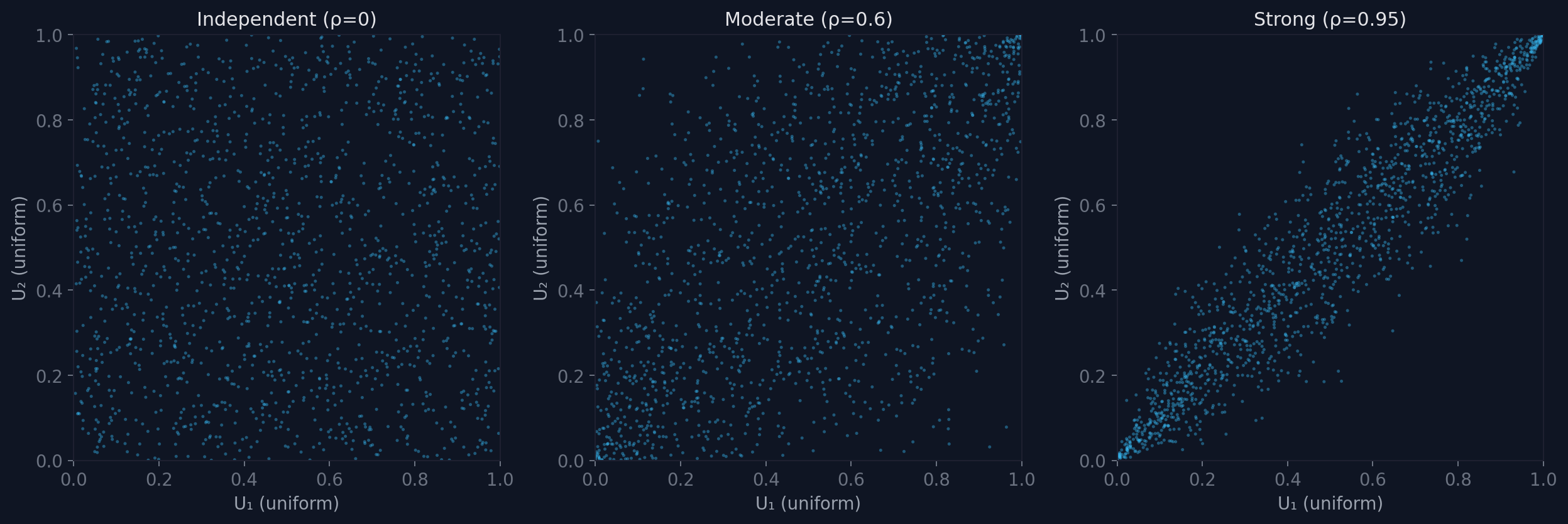
In this uniform space, independence looks like a uniform scatter across the unit square. Positive dependence clusters samples along the diagonal. Strong dependence compresses them into a narrow band.

This is the core insight. By working in [0,1]², we separate how much of each variable we observe (the marginals) from how they co-occur (the copula). The copula density c(u₁, u₂) tells us where in the unit square probability mass concentrates.

Diagonal convergence

As correlation increases, samples in copula space cluster progressively tighter along the diagonal. At the limit, perfect positive dependence (ρ → 1) means U₁ = U₂ always: every observation lies exactly on the diagonal. At perfect negative dependence (ρ → -1), samples lie on the anti-diagonal.

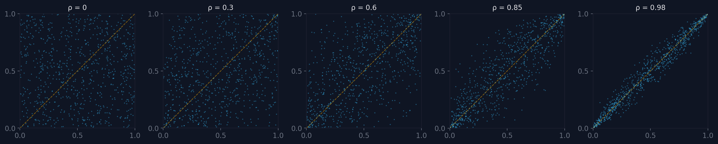
The rate and pattern of this convergence is exactly what the copula encodes. Different copula families converge differently: some compress symmetrically, others preferentially in one tail.

The Gaussian copula

The most widely used copula is derived from the multivariate Gaussian distribution. Transform each marginal to a standard normal, apply a correlation matrix, and transform back. The Gaussian copula has one parameter per variable pair: the linear correlation coefficient.

In 3D, the Gaussian copula density for a bivariate case with correlation 0.7 looks like this:

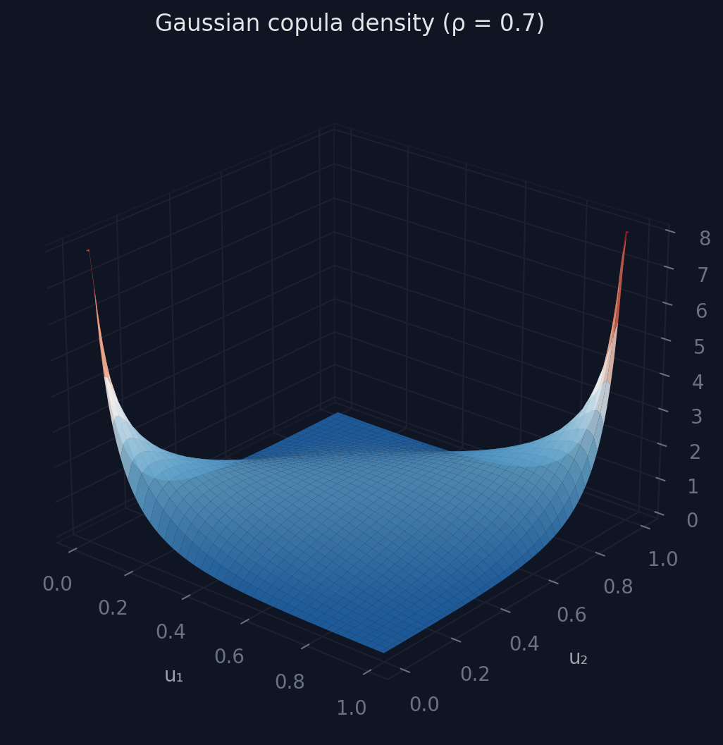
The ridges along the edges of the unit square show where the copula density is highest: the corners (0,0) and (1,1), where both variables are simultaneously low or simultaneously high. The 2D contour view makes the symmetry clearer:

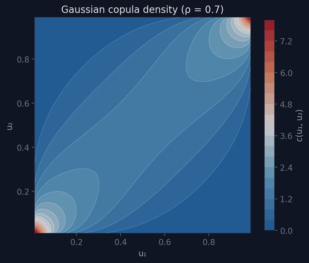
The Gaussian copula is symmetric: upper and lower tails have the same dependence structure. This is convenient but often wrong for climate data.

Copula families

Different copula families capture different dependence patterns. The three most important for climate risk:

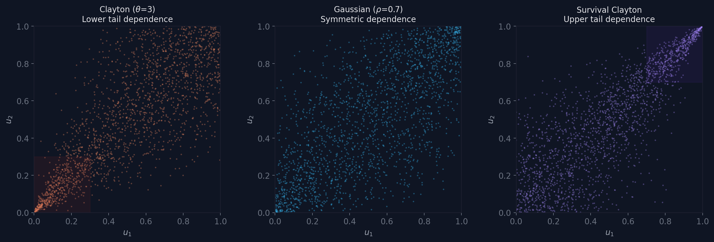
Clayton concentrates dependence in the lower tail. Both variables tend to be simultaneously low more often than simultaneously high. Useful for modelling joint deficit events (drought across multiple catchments, simultaneous low wind across a region).

Gaussian is symmetric. Upper and lower tails behave identically. Convenient as a default but rarely matches observed climate dependence.

Gumbel (and survival Clayton, shown here) concentrates dependence in the upper tail. Both variables tend to be simultaneously extreme. This is the pattern that matters most for compound hazards: storm wind and surge, heat and drought, heavy precipitation and saturated soil.

The 3D density surfaces make the asymmetry visible:

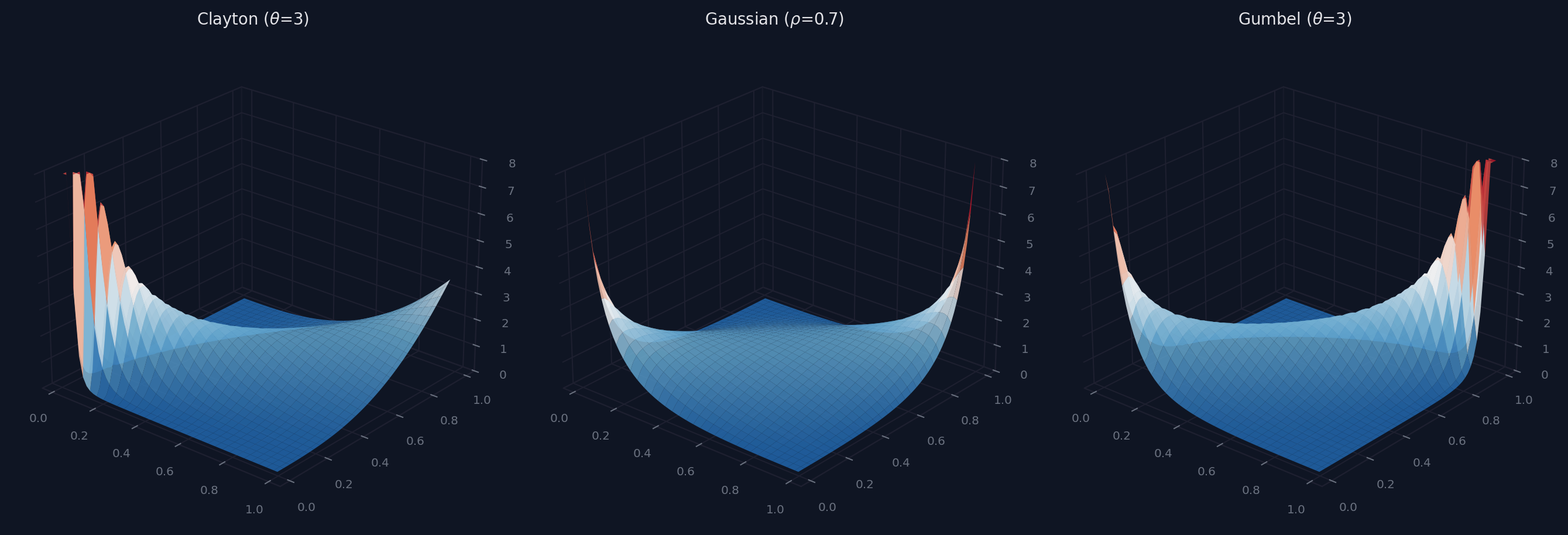
Clayton’s density spikes in the lower-left corner (0,0). Gumbel spikes in the upper-right (1,1). Gaussian spikes in both. For climate risk, the question is: does the data show symmetric dependence, or does the tail behaviour differ between extremes and normal conditions?

Explore it yourself

All three views below update together. Try this sequence:

1. Start with Gaussian at ρ=0.7. Note the symmetric ridges in the 3D surface, the elliptical scatter, and the balanced density heatmap.
2. Drag ρ toward 0.95. Watch the scatter compress onto the diagonal and the density peaks sharpen.
3. Switch to Clayton. The density mass drops to the lower-left corner. The scatter clusters near (0,0). This is lower-tail dependence: both variables tend to be simultaneously low.
4. Switch to Gumbel. The spike flips to the upper-right. The scatter fills the top-right quadrant. This is upper-tail dependence: the pattern that drives compound climate extremes.
5. Drag θ higher on Gumbel. The upper-tail concentration intensifies. This is what happens when you model correlated extremes properly instead of assuming independence.

Drag the 3D surface to rotate it. The heatmap (right, bottom) shows the same density from above.

Why tail dependence matters

Most of the time, it doesn’t matter which copula you use. The body of the distribution (moderate values) is similar across families. The differences emerge in the tails, where the data is sparse and the consequences are severe.

Same overall correlation, same marginals, but fundamentally different behaviour in the upper tail. The Gaussian copula produces far fewer joint extreme events than the upper-tail dependent structure. In a 1-in-100-year analysis, this difference is the difference between “rare but manageable” and “we needed more reinsurance.”

The effect compounds as you move deeper into the tail:

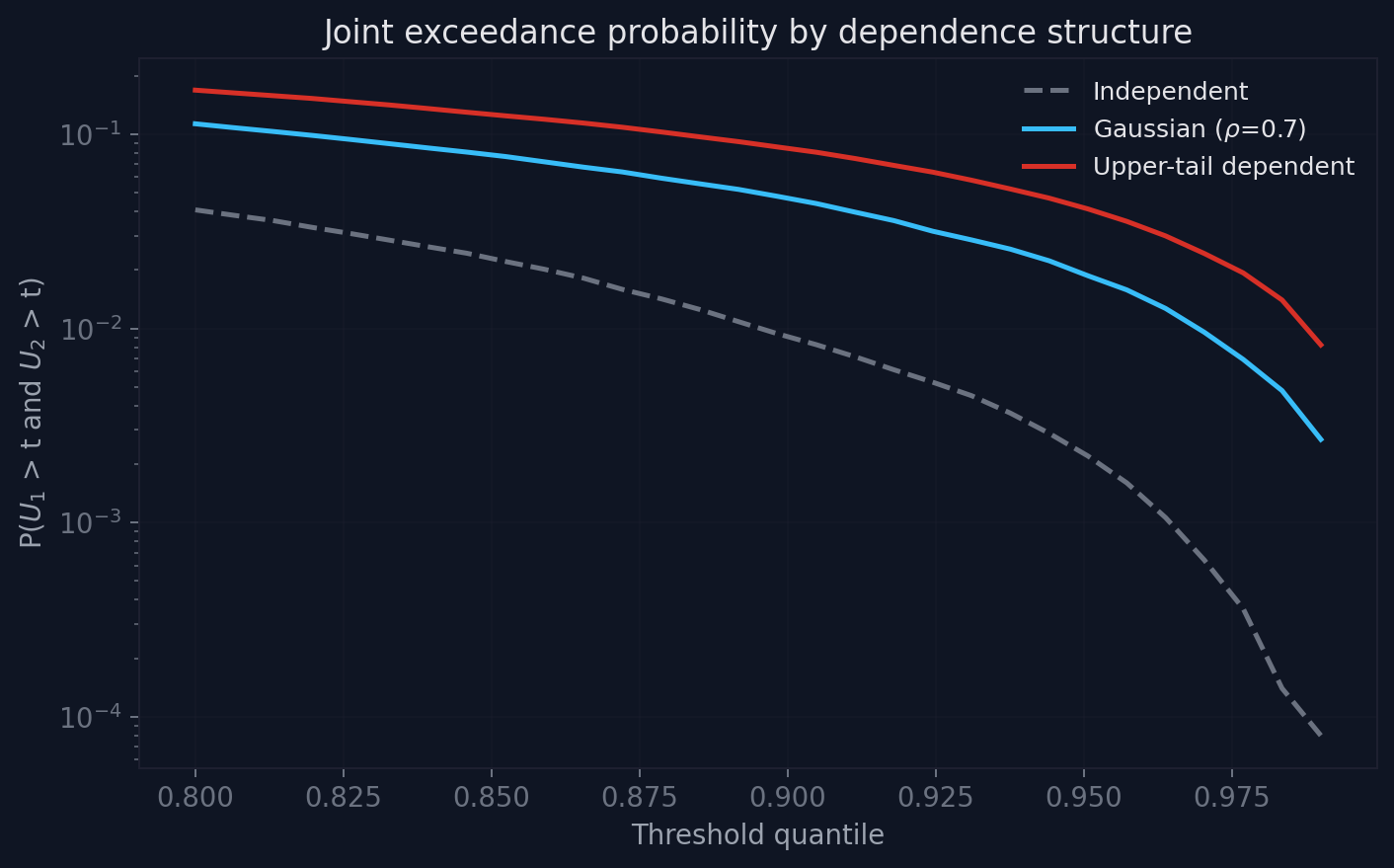
At the 95th percentile, the three structures differ by a factor of 2-3. At the 99th, by an order of magnitude. The independent assumption (dashed grey) is catastrophically wrong: it underestimates joint exceedance by 10x or more compared to the tail-dependent case.

This is why copula choice matters for reinsurance pricing. The difference between a Gaussian and a Gumbel copula, applied to the same marginals with the same correlation, can shift an aggregate loss estimate by billions.

Compound events in climate

The compound risk problem is not theoretical. European windstorms routinely produce correlated wind, rainfall, and surge. The 2013/14 UK winter storms, Storm Desmond (2015), and Storm Ciara (2020) all involved multiple simultaneously extreme hazards whose joint probability was far higher than independence would predict.

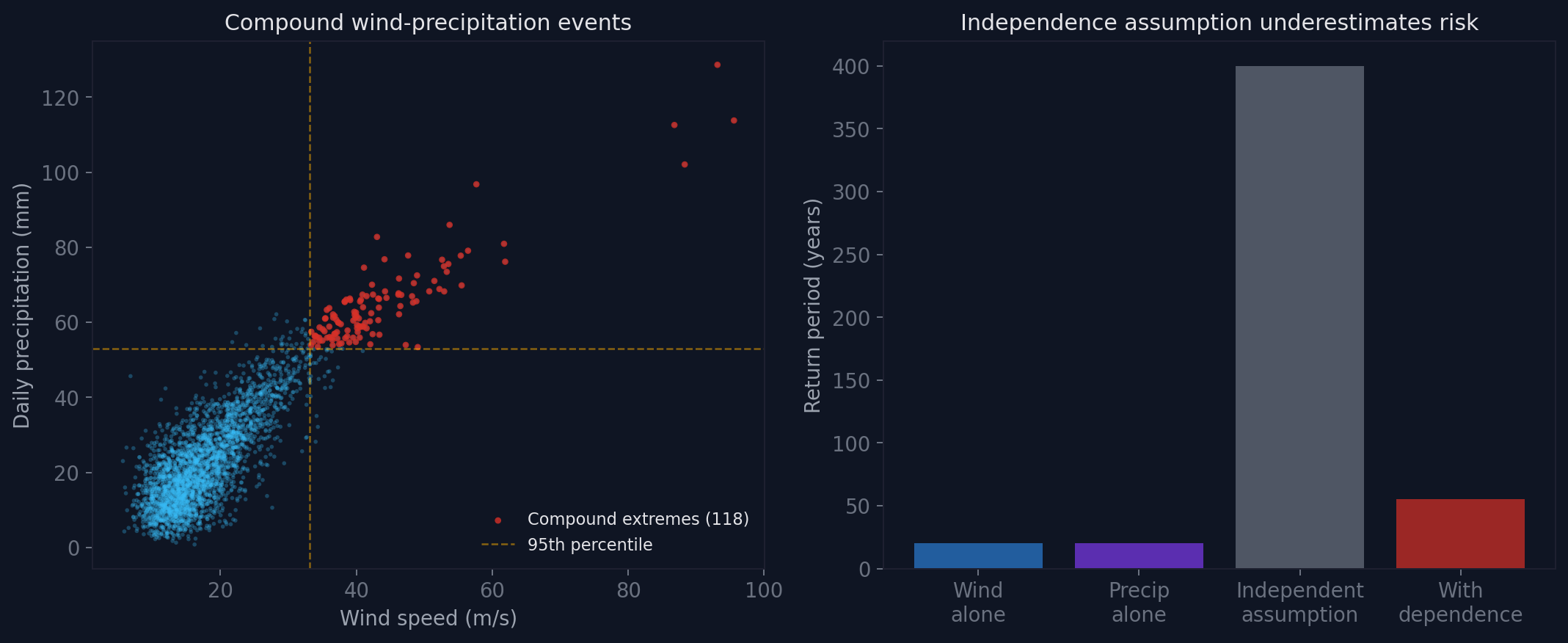
The left panel shows simulated wind-precipitation events drawn from an upper-tail dependent copula (survival Clayton, calibrated to be roughly consistent with observed winter storm co-occurrence). The red cluster in the upper right represents compound extremes where both hazards simultaneously exceed their 95th percentiles.

The right panel is the punchline. A 20-year wind event and a 20-year precipitation event, if independent, should co-occur once in 400 years. With realistic upper-tail dependence, the compound event has a return period closer to 55 years. Assuming independence underestimates the frequency by a factor of 7.

A typology of compound events

Zscheischler et al. (2020) defined four types of compound weather and climate events that are now standard in the literature:

Preconditioned events. A weather hazard whose impact is amplified by a preceding condition. Heavy rainfall on already-saturated soil produces far worse flooding than the same rainfall on dry ground. The antecedent condition (soil moisture) is not itself extreme, but it preconditions the system so that a moderate trigger produces a disproportionate response.

Multivariate events. Multiple hazards co-occurring at the same location and time. Storm surge combined with heavy precipitation during an extratropical cyclone. Concurrent heat and drought. High wind and intense rainfall. These are the events that copulas model most directly: the joint tail probability of two or more variables.

Temporally compounding events. A sequence where each event amplifies the impact of the next. Successive heatwaves without recovery time between them. Repeated flooding that prevents repair before the next event arrives. The dependence here is serial autocorrelation, not simultaneous co-occurrence.

Spatially compounding events. Multiple locations affected simultaneously, overwhelming response capacity even if no single location experiences an unprecedented event. Concurrent flooding across European river basins. Simultaneous crop failure in multiple breadbasket regions. The dependence is spatial correlation driven by large-scale atmospheric patterns.

Copulas are most directly relevant to the multivariate type, but they also appear in spatial compounding (modelling correlated extremes across locations) and in preconditioned events (modelling the dependence between the precondition and the trigger).

Zscheischler, J., Martius, O., Westra, S. et al. A typology of compound weather and climate events. Nat Rev Earth Environ 1, 333-347 (2020).

Beyond two variables

Real compound events rarely involve just two hazards. A coastal flood depends on wind speed, precipitation, storm surge, tidal state, and antecedent soil moisture. A heat-stress event involves temperature, humidity, and wind speed. The bivariate framework extends naturally to higher dimensions.

A trivariate Gaussian copula is parameterised by three pairwise correlations. You cannot visualise the density surface (that would require four dimensions), but you can visualise the samples as a point cloud in the unit cube and inspect the three pairwise projections.

The interactive visualisation below samples from a trivariate Gaussian copula with equal pairwise correlation. The threshold slider controls which points are flagged as joint exceedances (all three variables simultaneously above the threshold). Watch how:

1. At low ρ, the cube fills uniformly. Joint exceedances are rare and match the independent expectation.
2. As ρ increases, samples cluster along the main diagonal of the cube. Joint exceedances increase sharply.
3. The stats line shows the actual count vs the independent expectation. At high ρ and high thresholds, the ratio can exceed 10x.

The three pairwise scatter plots on the right show the marginal copula for each pair. Red points are those that exceed the threshold in all three variables, not just the two shown.

The trivariate case makes the compound risk argument viscerally clear. With three independent variables at the 90th percentile, joint exceedance is a 1-in-1000 event. With realistic dependence (ρ=0.6), it can be 1-in-50. That is a factor of 20 in risk that disappears if you assume independence.

What this means for risk modelling

Three practical implications:

Marginal analysis is necessary but not sufficient. Fitting marginal distributions to individual hazards tells you about the behaviour of each variable in isolation. It tells you nothing about co-occurrence. Any risk assessment that multiplies marginal exceedance probabilities is assuming independence, whether explicitly or not.

Copula choice is a modelling decision with large consequences. The Gaussian copula is the default in many applications (including, famously, pre-2008 CDO pricing). For climate risk, where upper-tail dependence is physically motivated (extreme wind drives extreme surge; atmospheric rivers produce both precipitation and wind), a symmetric copula systematically underestimates compound event frequency.

Data limitations are real. Fitting copulas to the tail requires tail data. By definition, extreme events are rare. Short observational records (50-100 years for most climate stations) provide limited information about joint tail behaviour. This is where physical understanding, reanalysis data (ERA5 provides 80+ years of gridded fields), and climate model ensembles become essential for constraining dependence in the tail.

---

This post covers the statistical framework. My dissertation applies these methods to specific compound extreme events across Europe using ERA5 reanalysis data. That work is ongoing and will be written up separately.