Building an Interactive GB Grid Scenario Tool from Public Data

Scotland generates more wind power than its transmission grid can carry south. The Scotland-England boundary (B6F in industry shorthand) is the single most constrained corridor in the GB network, and it gets worse every year as offshore wind capacity grows faster than reinforcement.

There is no public tool that lets you explore this. NESO publishes the data (network topology, boundary capabilities, generation projects, demand forecasts) but it lives in spreadsheets and PDFs. Commercial tools like PSS/E and PLEXOS cost tens of thousands of pounds and require weeks of training. If you’re a policy analyst, a student, a journalist, or a community energy group, you have no way to ask “what happens to the grid if Scottish wind doubles?” and get an answer in real time.

So I built one.

What the tool does

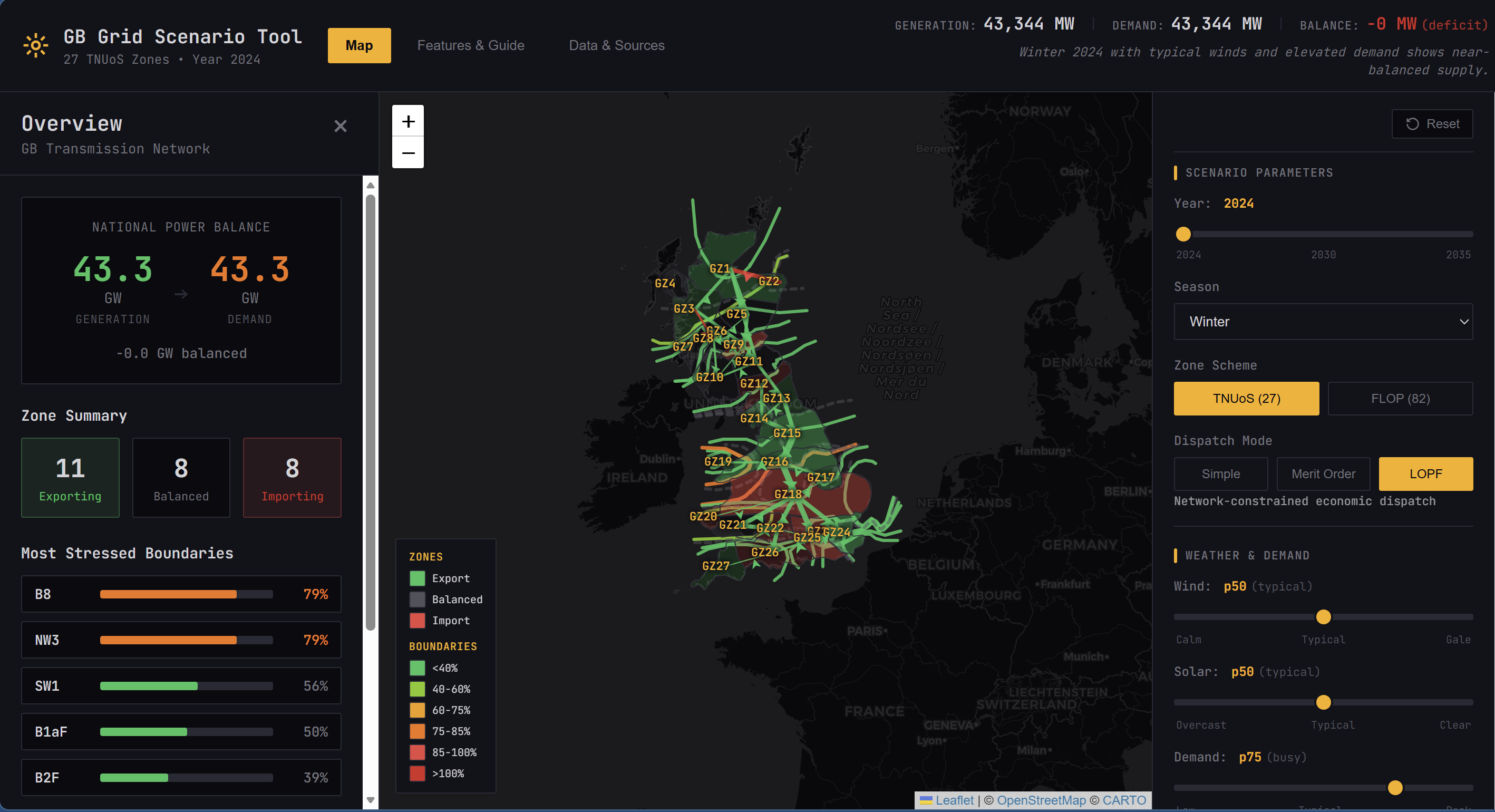
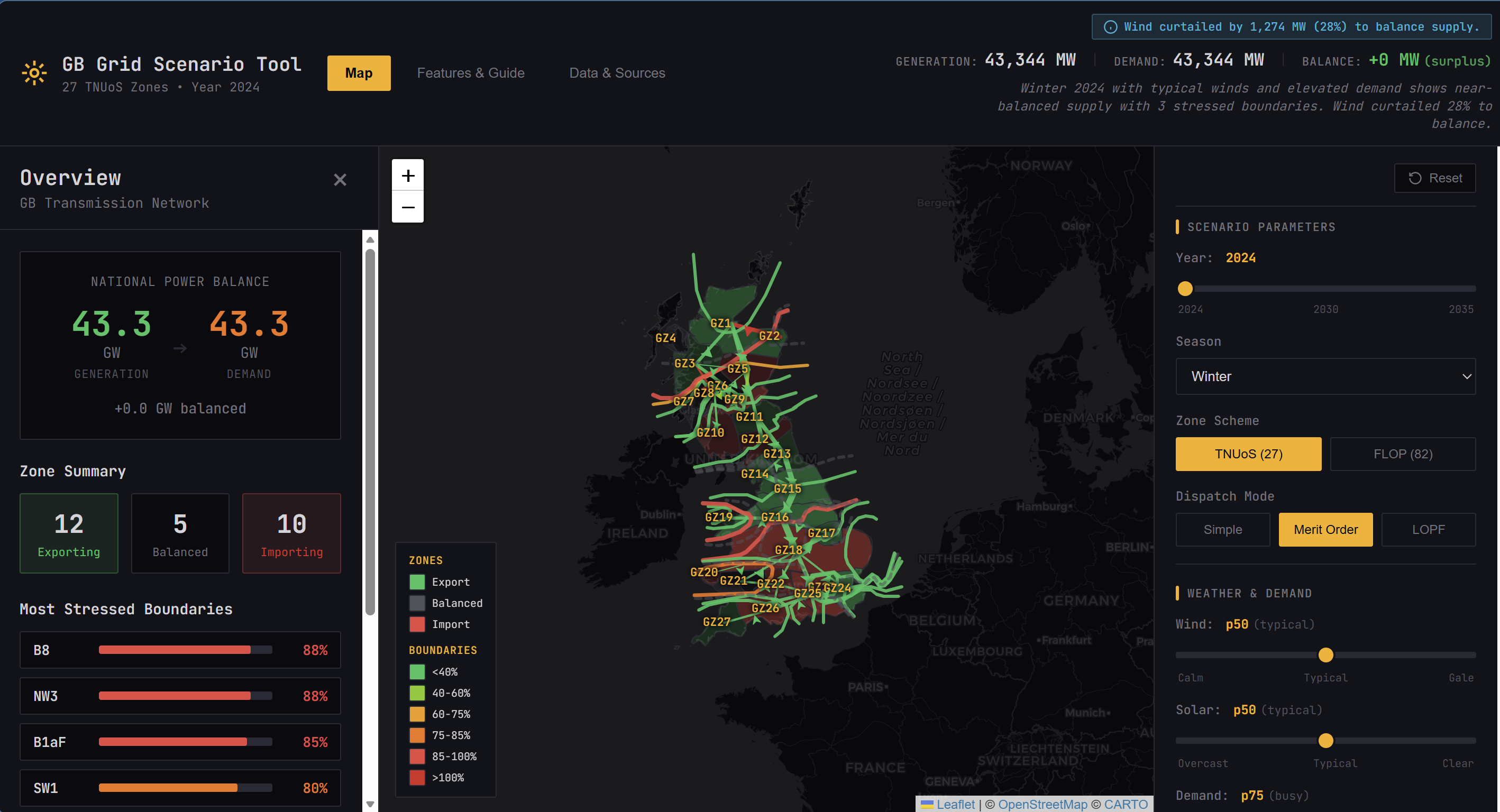
The GB Grid Scenario Tool is an interactive browser-based application for stress-testing the GB electricity transmission network. You select a year (2024-2035), choose a scenario, adjust weather sliders for wind, solar, and demand, toggle fuel types on or off, and see the results of a DC power flow calculation on a map with boundary utilisation heatmapping.

Three dispatch modes show the progression from naive to optimal:

Simple: all generation runs at full capacity. Shows raw generation potential but not realistic.
Merit order: generation dispatched cheapest-first until demand is met. Wind and solar run first, then gas fills the gap. Realistic cost ordering but ignores network constraints.
LP-optimal (LOPF): cost-minimised dispatch subject to boundary flow limits and per-link thermal constraints, solved using HiGHS compiled to WebAssembly. Closest to what NESO actually does operationally.

Under merit order dispatch at p73 wind, 9 of 18 mapped boundaries exceed their secure capability. Switch to LOPF and zero do. Same generation fleet, different allocation. That gap between unconstrained and constrained dispatch is what NESO spends billions managing every year through the Balancing Mechanism.

Everything runs client-side. No backend, no API calls, no account. Open a URL and start exploring.

Live demo (desktop recommended)

GB Grid Tool showing merit order dispatch with stressed boundaries

The validation journey

This is the part that doesn’t fit in a LinkedIn post but is where most of the engineering happened.

I validated against NESO’s published ETYS boundary transfer data: 75th and 95th percentile expected power flows across each boundary, by year and scenario. The target was B6F because it carries the dominant north-south transfer and has the most comparison data.

The demand baseline mistake

My first 10 configurations all had the same problem: every flow was 30-35% too high. I tried four network resolutions (27-zone, 82-zone, 137-zone hybrid, 674-node substation), two dispatch methods, two interconnector assumptions, reactance sensitivity analysis, circuit-level debugging. Nothing helped.

The root cause was embarrassingly simple. I was using ACS peak demand (47,940 MW), the design maximum that the grid is built to handle, instead of typical winter demand (~36,000 MW). One field in one JSON file. It inflated every injection by 34%, which inflated every flow proportionally.

The fix was one line. The investigation to find it took days.

Check your demand baseline before you optimise anything else.

16 configurations tested

After fixing demand, I tested systematically:

Resolution	Dispatch	IC mode	B6F error	Overall
27-zone TNUoS	Merit order	Dynamic IC	-2%	3 FAIR, 7 POOR
82-zone FLOP	Net injection	Dynamic IC	+13%	6 FAIR, 4 POOR
NESO 28-zone	Net injection	Dynamic IC	-15%	1 GOOD, 3 FAIR
137-zone hybrid	Various	Various	-3%	4 FAIR, 6 POOR

B6F within 2% is a real result. The remaining error on intermediate Scottish boundaries (B1aF, B2F, B3, typically 50-100% error) turned out to be fundamental, not fixable.

Why the remaining error exists

NESO uses PLEXOS, a commercial LP-based dispatch tool that distributes power using transfer sensitivities (how much a generator’s output change affects a specific boundary flow), not impedances. Their constraint model has no line reactances at all. Power is allocated by boundary flow limits, not by physics.

DC power flow does the opposite: it distributes power inversely proportional to impedance. Physically correct but produces different flow patterns from NESO’s LP.

Neither approach is wrong. DC power flow shows where power would flow if the network operated unconstrained. NESO’s model shows where power flows after active constraint management. The tool is most accurate for relative comparisons between scenarios (“what happens to B6 if Scottish wind doubles?”) where systematic biases cancel.

What I discovered along the way

NESO uses 82 internal “FLOP zones” for boundary analysis, not the 27 TNUoS zones they publish. I reverse-engineered the mapping from GSP boundary GeoJSON data and FES regional breakdown CSVs.
Real interconnector imports average 16.4% of capacity (1,611 MW), not the 65% commonly assumed. High GB demand correlates with high continental demand (cold weather across the North Sea region), reducing available imports.
Four ETYS boundaries (B0, NW1, NW2, SC3) sit at network edges (peninsulas and islands with no cross-zone link). They can’t be modelled at any zonal resolution.
The DC power flow engine was independently validated against PyPSA 1.1.2. All 43 link flows match to 0.000 MW.

Technical decisions

Why DC power flow, not AC? At 27-node zonal resolution, each node represents dozens of substations. Voltage magnitude and reactive power within a zone are meaningless at this aggregation. DC approximation captures the dominant physics (MW distribution by impedance) and is the same approximation NESO uses for boundary transfer analysis. AC would add complexity with no accuracy benefit.

Why merit order, not unit commitment? The tool runs single-timestep snapshots. Unit commitment requires temporal coupling: which generators were on last hour, start-up costs, ramp rates, minimum up/down times. That needs a backend or a fundamentally different architecture. Merit order with minimum stable level constraints is the best static approximation.

Why HiGHS in the browser? LOPF dispatch requires an LP solver. The alternatives: (a) send the problem to a backend server, (b) use a JavaScript LP library, (c) compile a production LP solver to WebAssembly. Option (a) adds infrastructure and latency. Option (b): the pure-JS solvers I tested couldn’t handle the problem size reliably. Option (c): HiGHS is a world-class open-source LP solver and compiles cleanly to WASM. Solve time is ~10ms for the 27-node problem. Instant feedback with no server dependency.

Why the SCADA theme? Every portfolio project uses Tailwind blue-on-white. The amber-on-black SCADA aesthetic communicates “this person understands how grids are operated” to anyone in the energy sector. It’s also more functional: high contrast, monospace fonts for data readability, flat panels matching real control room displays.

Why this tool exists, and what’s next

I built this tool because I needed a validated environment for RL dispatch research. The validation journey turned out to be bigger than expected, but the environment is now ready.

An earlier post trained agents with three national dispatch actions on scalar and spatial observations. They learned demand matching and merit order, but they could not learn network constraints because the action space had no spatial dimension. That work mapped the ceiling of action-space-limited RL on grid dispatch and motivated everything you see in this tool.

With the full 27-zone topology, the agent gets 109 continuous actions: per-zone per-type dispatch fractions with physical constraints. The same reward-focused agents, but now they can see the network and act on it. The next step is to test whether topology-aware actions let the agent learn what the LP solver computes analytically.

The hard part was building a validated environment from public data. That’s done.

The environment, the data, and the baselines are ready. The training infrastructure is the easy part.